while training an ml model, we all run into the age-old struggle of balancing the bias-variance tradeoff—it’s like trying to eat healthy while also craving dessert.

one of the techniques used in ml to lower both bias and variance at the same time is ensemble learning. okay, don’t let the term scare you—it’s actually a super simple concept.

ensemble learning is based on a very common idea called wisdom of the crowd. basically, instead of relying on a single model, we bring together multiple weak models (models that perform just a little better than random guessing), and somehow, they combine forces to create a much stronger and more accurate model. think of it like a group project where nobody is a genius, but together, they somehow manage to get an a.

ensemble learning is used in ml because:

better accuracy – multiple weak models combine to make a stronger, more accurate model. kinda like how a group of average students can somehow ace a project together.
reduces overfitting – individual models might overfit to specific data, but when combined, they generalize better. think of it as getting multiple opinions instead of trusting just one person.
handles bias-variance tradeoff – it helps balance bias (oversimplification) and variance (overfitting), making the model more reliable. basically, it’s the ml version of “work smarter, not harder.”
more robust predictions – since it takes input from multiple models, it’s less likely to make extreme mistakes. like how a jury makes better decisions than just one judge.

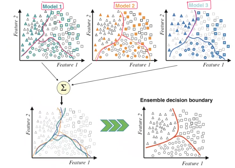
for example, this this image, we combine outputs from three different models to get a more accurate model.

now, lets look at some ensemble techniques:

1. voting

ensemble learning technique where multiple models “vote” to make a final prediction. By combining different models, the overall prediction is more reliable and robust. two types: voting classifier and voting regressor

voting classifier

each individual classifier in the ensemble predicts a class label, and the final prediction is made based on the majority vote (for classification tasks).

there are two types of voting:

hard voting: each model in the ensemble predicts a class label. The final prediction is the class that receives the majority of votes. for example, if three classifiers predict A, B, and A, the final prediction is A.
soft voting: each model predicts probabilities for each class. The final class is the one with the highest average probability. this method works best when the classifiers provide well-calibrated probabilities. for example, if the three classifiers predict class probabilities as follows:
- class A: 0.6, 0.3, 0.8
- class B: 0.4, 0.7, 0.2
the final prediction will be class A, as it has the highest average probability (0.6 + 0.3 + 0.8 = 1.7).

example: voting classifier (hard voting)

from sklearn.ensemble import VotingClassifier
from sklearn.linear_model import LogisticRegression
from sklearn.svm import SVC
from sklearn.tree import DecisionTreeClassifier
from sklearn.datasets import load_iris
from sklearn.model_selection import train_test_split

# Load dataset
data = load_iris()
X = data.data
y = data.target

# Split into train and test sets
X_train, X_test, y_train, y_test = train_test_split(X, y, test_size=0.3, random_state=42)

# Create individual classifiers
clf1 = LogisticRegression(max_iter=200)
clf2 = SVC(probability=True)
clf3 = DecisionTreeClassifier()

# Create a voting classifier (hard voting)
voting_clf = VotingClassifier(estimators=[('lr', clf1), ('svc', clf2), ('dt', clf3)], voting='hard')

# Train the model
voting_clf.fit(X_train, y_train)

# Evaluate the model
accuracy = voting_clf.score(X_test, y_test)
print(f"Voting Classifier Accuracy: {accuracy:.2f}")

voting regressor

the ensemble predicts continuous values. instead of selecting the majority vote, the final prediction is made by averaging the predictions of all the individual regressors.

example: voting regressor

from sklearn.ensemble import VotingRegressor
from sklearn.linear_model import LinearRegression
from sklearn.tree import DecisionTreeRegressor
from sklearn.svm import SVR
from sklearn.datasets import make_regression
from sklearn.model_selection import train_test_split

# Generate regression data
X, y = make_regression(n_samples=100, n_features=2, noise=0.1, random_state=42)

# Split into train and test sets
X_train, X_test, y_train, y_test = train_test_split(X, y, test_size=0.3, random_state=42)

# Create individual regressors
reg1 = LinearRegression()
reg2 = DecisionTreeRegressor(random_state=42)
reg3 = SVR()

# Create a voting regressor
voting_reg = VotingRegressor(estimators=[('lr', reg1), ('dt', reg2), ('svr', reg3)])

# Train the model
voting_reg.fit(X_train, y_train)

# Evaluate the model
score = voting_reg.score(X_test, y_test)
print(f"Voting Regressor R-squared: {score:.2f}")

2. bagging

when we want to improve the performance of our machine learning models, we often look to ensemble techniques. bagging, pasting, random patches, and subspaces are all variations of ensemble learning that use multiple models to make better predictions. let’s break them down in simple terms.

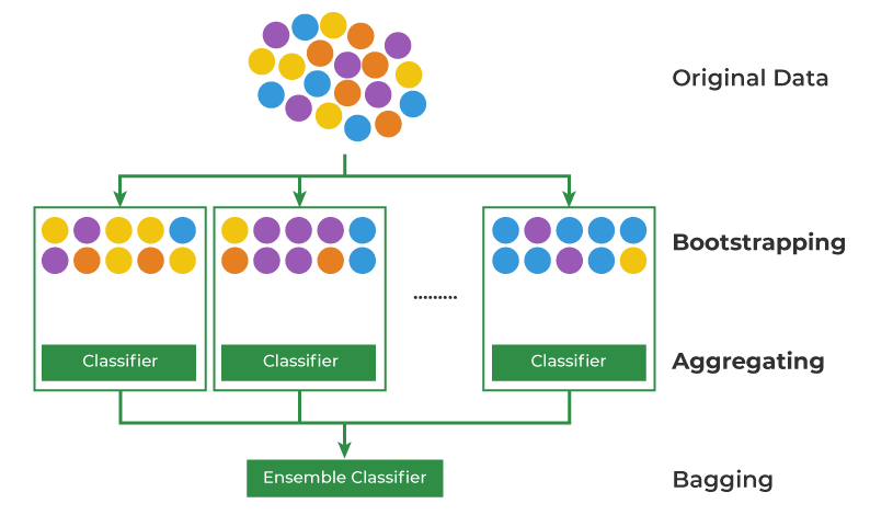
bagging (bootstrap aggregating)

bagging stands for bootstrap aggregating, which is a technique where we train multiple models on different random samples of the data (with replacement) and then combine their predictions. the idea is that each model will see a slightly different view of the data, and combining their predictions will make the final model more robust.

how it works:

random samples of the data (with replacement) are used to train different models.
the final prediction is typically made by averaging the predictions for regression or taking a majority vote for classification.

example: bagging with decision trees

from sklearn.ensemble import BaggingClassifier
from sklearn.tree import DecisionTreeClassifier
from sklearn.datasets import load_iris
from sklearn.model_selection import train_test_split

# load dataset
data = load_iris()
X = data.data
y = data.target

# split into train and test sets
X_train, X_test, y_train, y_test = train_test_split(X, y, test_size=0.3, random_state=42)

# create a base classifier
base_clf = DecisionTreeClassifier()

# create a bagging classifier
bagging_clf = BaggingClassifier(base_clf, n_estimators=50)

# train the model
bagging_clf.fit(X_train, y_train)

# evaluate the model
accuracy = bagging_clf.score(X_test, y_test)
print(f"bagging classifier accuracy: {accuracy:.2f}")

3. boosting

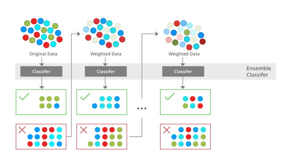
sequential ensemble method where each model is trained to correct the mistakes made by the previous one. instead of training models independently, boosting trains models one after another, focusing more on the samples that were misclassified by earlier models. over time, boosting creates a strong model from a combination of weak learners (models that perform slightly better than random chance).

how it works:
1. train the first model.
2. identify the errors made by the first model and assign higher weights to those samples.
3. train the next model on the data with the updated weights.
4. repeat the process, adding more models that focus on fixing the mistakes of the previous ones.

from sklearn.ensemble import AdaBoostClassifier
from sklearn.tree import DecisionTreeClassifier
from sklearn.datasets import load_iris
from sklearn.model_selection import train_test_split
from sklearn.metrics import accuracy_score

# Load the dataset
data = load_iris()
X = data.data
y = data.target

# Split the data into training and testing sets
X_train, X_test, y_train, y_test = train_test_split(X, y, test_size=0.3, random_state=42)

# Initialize and train the AdaBoost model
base_model = DecisionTreeClassifier(max_depth=1)  # weak model
model = AdaBoostClassifier(base_model, n_estimators=50, random_state=42)
model.fit(X_train, y_train)

# Make predictions
y_pred = model.predict(X_test)

# Evaluate the model
print(f"Accuracy: {accuracy_score(y_test, y_pred):.4f}")

famous examples:
- adaboost: adds weights to misclassified samples so the next model focuses on them. it’s one of the earliest and most well-known boosting algorithms.
- gradient boosting: builds new models to correct the residuals (errors) of the previous models. each new model focuses on fixing the prediction errors of the last one.
- xgboost: a more efficient and scalable version of gradient boosting, often used in machine learning competitions for its strong performance.

4. stacking (stacked generalization)

ensemble method where different types of models (not just the same one) are trained, and their predictions are combined by a meta-model. the idea is that different models may capture different aspects of the data, so by combining their predictions, you get the best of all worlds. after the base models make their predictions, a final meta-model is trained to make the final decision using the outputs of the base models.

how it works:
1. train multiple different base models (like decision trees, logistic regression, or neural networks) on the data.
2. the predictions of these base models are used as input features for the next step.
3. train a meta-model on these predictions to make the final prediction.

from sklearn.ensemble import StackingClassifier
from sklearn.linear_model import LogisticRegression
from sklearn.tree import DecisionTreeClassifier
from sklearn.svm import SVC
from sklearn.datasets import load_iris
from sklearn.model_selection import train_test_split
from sklearn.metrics import accuracy_score

# Load the dataset
data = load_iris()
X = data.data
y = data.target

# Split the data into training and testing sets
X_train, X_test, y_train, y_test = train_test_split(X, y, test_size=0.3, random_state=42)

# Define the base models
base_models = [
    ('decision_tree', DecisionTreeClassifier()),
    ('svc', SVC(probability=True)),
    ('logistic', LogisticRegression())
]

# Define the meta-model
meta_model = LogisticRegression()

# Initialize the stacking model
model = StackingClassifier(estimators=base_models, final_estimator=meta_model)
model.fit(X_train, y_train)

# Make predictions
y_pred = model.predict(X_test)

# Evaluate the model
print(f"Accuracy: {accuracy_score(y_test, y_pred):.4f}")

famous use case:
stacking is often used when you want to combine the strengths of different types of models. for example, combining decision trees (which are great at handling categorical data) with logistic regression (which can handle continuous data) can yield a better model.